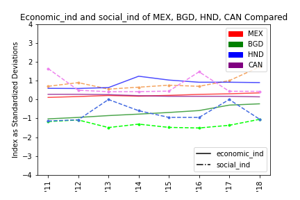
Visualization of index change over time
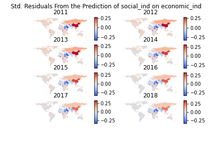
Visualization of residuals from the regression of social empowerment on economic empowerment
This page highlights my work on a group project analyzing women's economic empowerment as a driver of social empowerment. Given empowerment an abstract concept, our team sought to index these values for ease of analysis. Following is the code used to define the project's indices for multiple hypothesis testing. Also included is the code to regress economic empowerment on social empowerment.
Inspiration for variables stems from the UNDP's Gender Inequality Index, data was collected using the World Bank's API using the WBGAPI library for Python, and methodology follows from Anderson 2008 and Schwab et al 2021.
			# ### Creating indices

	# Inverts signs for variables as needed such that a positive sign indicates a
	# positive outcome.
	def invert_sign(df, vars_and_signs):
	    for var in vars_and_signs:
	        if vars_and_signs[var] == True:
	            df[var] = df[var] * -1
	    return(df)

	# Standardizes to a std. deviation score for each var.
	def standardize(df, variables):
	    # Removes keys from dictionary in cases where dictionaries are used to define
	    # variable sign

	    if type(variables) == dict:
	        variables = list(variables.keys())
	    elif type(variables) == str:
	        variables = list(variables)


	    # Demean all k, subtract mean of the indicator in the reference group
	    for var in variables:
	        meanvar = df[var].mean()
	        stdvar = df[var].std()
	        df['STD.{}'.format(var)] = df[var].apply(lambda x: (x-meanvar)/stdvar)

	    return(df)


	# Takes standardization and applies it across years so we get year-effects
	# rather than a mess of near-unstandardized values.
	def standardize_by_year(df, variables, weighting, inc_weights):
	    stack_df = pd.DataFrame()

	    # Takes it BY year and standardizes each variable to that year to capture
	    # by-year effects.
	    for yr in list(df['year'].unique()):
	        wdf = df[df['year'] == yr]

	        wdf = standardize(wdf,variables)

	        # Functionality to use for pre- and post-weighting
	        if weighting:
	        # Weight_vars to weight and then stack
	            std_vars = [col for col in list(wdf.columns) if 'STD' in col]
	            wdf = weight_vars(wdf, std_vars, inc_weights)

	        # Stack DFs by year
	        stack_df = pd.concat([stack_df,wdf])

	    return(stack_df)


	# Weights vars based on inverse covariance, following Anderson (2008) and
	# Schwab et al. (2021) who formalize the function for Stata

	def weight_vars(df, std_vars, inc_weights):
	    # Get the inverse of the covariance matrix, sum across rows to get weight
	    inv_cov_mat = np.linalg.inv(df[['economy','year'] + std_vars].cov())
	    weights = list(sum(inv_cov_mat))

	    # Uses dictionary and list comprehension to build a dictionary of matched
	    # dictionary and weight values
	    var_weight_matches = {var:weight for (var, weight) in
	                          [(var, weight) for (var, weight) in zip(std_vars, weights)]
	                          }

	    for var in std_vars:
	        # new var named to indicate weighting
	        df['Wgt.{}'.format('.'.join(var.
	                                    split('.')[1:3]))] = df[var] * var_weight_matches[var]
	        if inc_weights:
	            df['Wgt.AMT.{}'.format('.'.join(var.split('.')[1:3]))] = var_weight_matches[var]
	    return(df)

	    # Weight the indicators by the weights for each group (which is each year)
	    # sum the weighted averages.

	    # Variable weight based on order of variable entry, [var1, var2] will be
	    # [entry1,entry2], respectively, in the sum of each row.

	# Pulls column names with the % weight by variable for validation.
	# - Optional but good to see how variables are weighted based on the inv. cov. matrix.
	def get_weighted_cols(df):
	    w_vars = [col for col in list(df.columns) if 'Wgt' in col]
	    weight_cols = []
	    for weight_var in w_vars:
	        try:
	            weight_cols.append(re.search('^Wgt.(?!.*AMT).+$',weight_var).group())
	        except AttributeError:
	            pass
	    return(weight_cols)

	    # Check AMT doesn't follow - regex:
	    # https://stackoverflow.com/questions/32862316/negative-lookahead-with-capturing-groups

	# Final index creation, inverting, weighting, standardizing, creating the index,
	# re-standardizing, and outputting.
	def create_index(df, vars_and_signs, treatment_group, index_name,
	                 inc_stdized=False, inc_weights=False):

	    # vars_and_signs MUST be a dictionary
	    if type(vars_and_signs) != dict:
	    # eg. vars_and_signs: {'var1':True,'var2':False} will invert var1
	    # but not var2
	        raise ValueError('vars_and_signs MUST be dictionary')
	    # Invert score needs to offer options by variable

	    # Indicating "treatment"
	    working1 = df
	    working1['e'] = working1['economy'].map(lambda x:
	                                            1 if x in treatment_group else 0)

	    # Inverting sign by need
	    working1 = invert_sign(working1,vars_and_signs)

	    # Indicator normalization
	    wdf = standardize_by_year(working1, vars_and_signs, True, inc_weights)

	    # Dragging out column names for later addition
	    std_vars = [col for col in list(wdf.columns) if 'STD' in col]
	    weight_cols = get_weighted_cols(wdf)

	    # Index creation (weighted sum of indicators)
	    wdf[index_name] = wdf[weight_cols].sum(axis = 1)

	    # Index normalization
	    wdf = standardize_by_year(wdf,[index_name], False, inc_weights)
	    wdf[index_name] = wdf['STD.{}'.format(index_name)]
	    wdf['year'] = wdf['year'].apply(lambda x: int(x.replace('YR','')))

	    if inc_weights:
	        if inc_stdized:
	            return(wdf[['economy','year','e',index_name]
	                       + weight_cols + std_vars])
	        else:
	            return(wdf[['economy','year','e',index_name] + weight_cols])
	    else:
	        if inc_stdized:
	            return(wdf[['economy','year','e',index_name] + std_vars])
	        else:
	            return(wdf[['economy','year','e',index_name]])

# ### Statistical Modeling functions

def categorize_std_deviations(variable):
    if -0.5 <= variable <= 0.5:
        return('Between -0.5 and 0.5')
    elif -1.5 <= variable < -.5:
        return('Between -1.5 and -0.5')
    elif -2.5 <= variable < -1.5:
        return('Between -2.5 and -1.5')
    elif variable < -2.5:
        return('Less than -2.5')
    elif 0.5 < variable <= 1.5:
        return('Between 0.5 and 1.5')
    elif 1.5 < variable <= 2.5:
        return('Between 1.5 and 2.5')
    elif variable > 2.5:
        return('Greater than 2.5')

def model_ols(df, dependent, independent,
              country_override='', return_signif=False):

    ols_df = pd.DataFrame({'Country':[],'Coefficient':[],'P-Value':[]})

    if country_override != '':
        df[df['economy'] == country_override]

    country_list = list(df['economy'].unique())


    for i in range(len(country_list)):
        wdf = df[df['economy'] == country_list[i]]

        x = wdf[[independent]].values
        y = wdf[[dependent]]

        X = sm.add_constant(x)
        model = sm.OLS(y,X)
        results = model.fit()

        ols_df.loc[i] = [country_list[i], results.params[1], results.pvalues[1]]

    # Creating an indicator for negativeness to count the inversions of expectation.
    ols_df['is_negative'] = ols_df['Coefficient'].apply(lambda x:
                                                        1 if (x <0) else 0)

    if return_signif:
        return(ols_df[ols_df['P-Value'] <= 0.05])

    return(ols_df)


def map_residuals(df, dependent, independent, year_override=2018,
                  return_df=False, multi_year=False, save_fig=False):
    # Following the process of ArcGIS' residual mapping procedures, we create a regression model that,
    # by year, can present model accuracy.
    # Allows for multiple charts or a single, interactive chart depending on the context.

    wdf = df
    if multi_year:
        year_list = wdf['year'].unique()
        subs = int(len(year_list)/2)
        fig, ax = plt.subplots(subs, 2)
    else:
        subs = 1
        fig, ax = plt.subplots()
        wdf = df[df['year'] == year_override]


    world = gpd.read_file(gpd.datasets.get_path('naturalearth_lowres'))

    x = wdf[[independent]].values
    y = wdf[[dependent]]

    X = sm.add_constant(x)
    model = sm.OLS(y, X)
    wdf['residuals'] = model.fit().resid

    # Comparing residuals to our index, categorizing predicted against actual
    # by std. deviations. Good news: our index is already in
    # std. deviations so we can compare directly.

    wdf['dist_from_actual'] = wdf[dependent] - wdf['residuals']
    wdf['dist_cat'] = wdf['dist_from_actual'].apply(lambda x:
                                                    categorize_std_deviations(x))

    if return_df:
        return(wdf)

    # Merging the residual dataset with the world df and mapping.
    world_indexes = world.merge(wdf, left_on = 'iso_a3', right_on = 'economy')

    if multi_year:
        # Iterates by year to make multiple subplots

        year_iterators = [i for i in range(round(len(year_list)/2)) for _ in (0, 1)]
        axes_iterators = [0,1] * len(year_list)
        for i in range(len(year_iterators)):

            # Turns our indexed ax into a variable for cleaner use later
            ax_object = ax[year_iterators[i]][axes_iterators[i]]

            year_df = world_indexes[world_indexes['year'] == year_list[i]]

            # Creates a properly-scaled color axis object/colormap bar
            # on the proper end of the graph
            divider = make_axes_locatable(ax_object)

            cax = divider.append_axes('right', size='5%', pad = 0.1)

            year_df.plot(ax = ax_object, column = year_df['dist_from_actual'],
                               legend = True, cmap = 'coolwarm', cax = cax)

            ax_object.axis('off')
            ax_object.set_title(year_list[i])
        fig.suptitle('Std. Residuals From the Prediction of {} on {}'.
                     format(dependent, independent))

    else:
        world_indexes.plot(ax = ax, column = world_indexes['dist_from_actual'],
                           legend = True, cmap = 'coolwarm', cax = cax)

        ax.set_title('Std. Residuals From the Prediction of {} on {} in {}'.
                     format(dependent, independent, str(year_override)))
        ax.tick_params(left = False, right = False , labelleft = False ,
                    labelbottom = False, bottom = False)

    if save_fig:
        fig.savefig(WD + '/' + 'residual_map_all_years.png')


def get_reg_summary(reg_df, signif_val=0.05):

    signif_df = reg_df[reg_df['P-Value'] <= signif_val]
    num_signif = len(signif_df)
    percent_signif = len(signif_df) / len(reg_df)
    num_negative = reg_df['is_negative'].sum()
    percent_negative = reg_df['is_negative'].sum() / len(reg_df)
    num_neg_signif = signif_df['is_negative'].sum()
    percent_neg_signif = signif_df['is_negative'].sum() / len(signif_df)

    summ_df = pd.DataFrame({'Num Signif':[num_signif],
                            'Percent Signif': [percent_signif],
                            'Num Negative': [num_negative],
                            'Percent Negative': [percent_negative],
                            'Num Neg + Signif':[num_neg_signif],
                            'Percent Neg + Signif':[percent_neg_signif]})
    return(summ_df)
Below, I feature some of the output from the above code, including visualization of the indices across the project's primary countries of interest and the comparison state, Canada, as well as the mapped residuals.
Visualization of index change over time
Visualization of residuals from the regression of social empowerment on economic empowerment